Exploring Unusual Options activity with Python and APIs

Unraveling market mysteries with Intrinio’s options data APIs

Introduction

Options data for stocks can be valuable if one understands how to utilize it properly. This article will explore using the Intrinio EOD Historical Options endpoint in Python to import and analyze unusual options data. I will assume the reader is familiar with trading or investing in Options. Let’s dive right in.

Unusual Options Activity

There are a few formal definitions; however, unusual options activity usually refers to an abnormal increase in the trading volume of an options contract. What would constitute an abnormal increase in trading volume? We will discuss that further once we get into coding this out in Python. With options, we can use two metrics to understand trading volume: Open Interest & Volume. Check out the formal definitions below from Investopedia:

Open Interest definition from Investopedia

Open interest is the total number of outstanding derivative contracts for an asset — such as options or futures — that have not been settled.

Volume definition from Investopedia

For options markets, the volume metric tabulates the number of options contracts bought or sold on a given trading day; it also identifies the activity level for a particular contract.

It is essential to understand these two distinct differences. Open Interest shows how many parties hold an options contract, while Volume shows how many contracts were traded in a day.

For example, let’s say there are currently 100 sets of parties holding call option contracts for a particular strike and expiration date at the end of the trading day for AAPL. Open Interest for that particular contract would be 100. On the other hand, this same contract was bought and sold between 1000 sets of parties on the same day. Therefore, Volume would be 1,000 at the end of the trading day.

Now that we have established what unusual options activity is and the key metrics we will be isolating to explore it, let’s dive into the data with Intrinio and Python!

Libraries

For this exercise, we will use several different Python libraries. As we work through each step, I’ll explain which library is being used and why. You may need to install some of these if you follow along.

import yfinance as yf
import re
import pandas as pd
from datetime import datetime, timedelta
import requests
from tqdm import tqdm
import seaborn as sns
import matplotlib.pyplot as plt
sns.set()

Importing the Data

With options data, there will be exponentially more bytes of actual data compared to a stock’s standard open, high, low, and close price data. For each market day, you have your standard close prices for each stock; however, each stock with options will have thousands of contracts and the corresponding data related to those contracts. In addition, we are looking at historical options data, which will compound the sheer amount of data we will use.

Note that we will be using the stock AAPL to demonstrate this workflow. We will start by importing the option contract symbols, as the Intrino EOD options API requires specific option symbols to pull the historical data. We will use the yfinance library to pull the symbols, which pulls data straight from Yahoo Finance. I’ve built a function that accomplishes this and outputs a DataFrame of the option contract symbols for a given stock.

def get_options_data(ticker):
    try:
        stock = yf.Ticker(ticker)
        options_dates = stock.options
        all_data = []
        for expiration_date in options_dates:
            options = stock.option_chain(expiration_date)
            calls = options.calls
            puts = options.puts
            for _, call in calls.iterrows():
                all_data.append({'Symbol': call['contractSymbol']})
            for _, put in puts.iterrows():
                all_data.append({'Symbol': put['contractSymbol']})
        return pd.DataFrame(all_data)
    except Exception as e:
        print(f"Error occurred: {e}")
        return None

options_symbol_data = get_options_data(ticker = 'AAPL')

Next up, we will import the historical OHLC prices for AAPL using the yfinance library.

def get_historical_price_data(ticker):
    try:
        stock = yf.Ticker(ticker)
        data = stock.history(period="max")
        data.index = data.index.strftime('%Y-%m-%d')
        return data
    except Exception as e:
        print(f"Error occurred: {e}")
        return None

ohlc_prices = get_historical_price_data(ticker = 'AAPL')

We now have our historical stock price data and option symbols. Next, we must import our historical EOD option data with Intrinio’s EOD historical options data API. Note that you will need an API key to use this. When writing this, we have close to 2,000 various option symbols for which to pull data.

When importing this data, we will also need to extract the following information for each contract: strike price, days to expiration, and whether or not it is a call or put. We will do this by using regular expressions on the actual contract symbol. Let’s review the anatomy of an option contract symbol for reference.

Take this one as an example: AAPL240510C00100000. This symbol is for an AAPL call expiring on 05–10–2024 with a strike price of $100. The first part of the symbol represents the underlying stock symbol. The next 6 digits represent the date. The letter following the date indicates whether or not it is a call or a put. Lastly, the next 8 digits represent the strike price. The next set of functions is used in tandem to extract this information and the historical option price data.

def Extract_Expiration_Date(text):
    pattern = r'^[A-Z]+(\d{6})[A-Z]+\d{5}\d+'
    match = re.search(pattern, text)
    if match:
        captured_digits = match.group(1)
        transformed_string = '20' + captured_digits[:2] + '-' + captured_digits[2:4] + '-' + captured_digits[4:]
        return pd.to_datetime(transformed_string)
    else:
        return None

def extract_strike(option_string):
    # Use regular expression to extract the last 8 digits
    match = re.search(r'\d{8}$', option_string)
    if match:
        number_str = match.group()
        # Insert decimal and remove leading zeroes
        number_str = number_str[:-3].lstrip('0') + '.' + number_str[-3:]
        return float(number_str)
    else:
        return None

def historical_eod_options_data(contract_symbol, api_key):
  try:
    url = f'https://api-v2.intrinio.com/options/prices/{contract_symbol}/eod?api_key={api_key}'
    eod_options_json = requests.get(url).json()
    df = pd.DataFrame(eod_options_json['prices'])
    df_sorted = df.sort_values(by='date', ascending=True).reset_index(drop=True)
    df_sorted = df_sorted[['date','open_interest','volume']]
    
    ## Add expire date
    expire_date = Extract_Expiration_Date(contract_symbol)
    df_sorted['date'] = pd.to_datetime(df_sorted['date'])
    df_sorted['DTE'] = (expire_date - df_sorted['date']).dt.days

    ## Strike Price
    strike = extract_strike(contract_symbol)

    ## Option Type
    match = re.search(r'.{8}(.).{8}$', contract_symbol)
    option_type = match.group(1)

    ## Add New Columns
    df_sorted['Strike'] = strike
    df_sorted['Option_Type'] = option_type
    df_sorted['DTE'] = (expire_date - df_sorted['date']).dt.days

    return df_sorted
  except Exception as e:
    print(f"Error occurred: {e}")
    print(f"Contract format incorrect or does not exist on this date")
    return None

Next, we will use these functions to import the historical data for all option contracts. It looks like a fairly straightforward script, but note we are importing a large amount of data. In total, this script took my machine about seven minutes to run. We will also include the historical close prices of the underlying stock and use this information to say whether each option was in-the-money or out-of-the-money on each trading day. I find the tqdm library helpful here as I like to see how long the script takes to run.

hist_options_dfs = []
api_key = 'YOUR_API_KEY_HERE'

for i in tqdm(range(len(options_symbol_data))):
  s = options_symbol_data['Symbol'][i]
  hist_data = historical_eod_options_data(contract_symbol = s,api_key = api_key)
  hist_options_dfs.append(hist_data)\

hist_option_df = pd.concat(hist_options_dfs).reset_index(drop=True)

hist_option_df['date'] = pd.to_datetime(hist_option_df['date'])
ohlc_prices.index = pd.to_datetime(ohlc_prices.index)
ohlc_prices = ohlc_prices[['Close']]
merged_df = pd.merge(hist_option_df, ohlc_prices, left_on='date', right_index=True, how='left')

merged_df['Moneyness'] = None

for i in tqdm(range(len(merged_df))):
  option_type = merged_df['Option_Type'][i]
  strike = merged_df['Strike'][i]
  close = merged_df['Close'][i]
  if (option_type == 'C') & (strike > close):
    merged_df['Moneyness'][i] = 'otm'
  elif (option_type == 'P') & (strike > close):
    merged_df['Moneyness'][i] = 'itm'
  elif (option_type == 'C') & (strike < close):
    merged_df['Moneyness'][i] = 'itm'
  else:
    merged_df['Moneyness'][i] = 'otm'

Exploring the Data

Our data is now imported, so it’s time to explore it. When exploring data, I believe it is important to have a specific goal in mind; in this case, I want to explore if the options with the highest day-over-day changes in open interest and/or volume lead to higher volatility/returns in the underlying stock price over the following trading day. It will be valuable to break this down by the moneyness and the type of options (calls or puts).

To explore the data in this matter, we will have to reformat it. This will involve several steps, which I will mention below in addition to the code that goes along with it:

1. Create four groups of data by moneyness and type.
2. Calculate the average open interest and volume per contract using each subset. Note that we are doing this on a per-contract basis. This is a way of normalizing the data because the contracts we are currently looking.
3. Calculate the day-over-day changes in each of these metrics.
4. Calculate the next day’s return in the underlying price.
5. Merge the data and visualize.

# Filter observations where 'Moneyness' is 'itm' and 'Option_Type' is 'C' (in-the-money calls)
itm_calls_df = merged_df[(merged_df['Moneyness'] == 'itm') & (merged_df['Option_Type'] == 'C')]

# Filter observations where 'Moneyness' is 'itm' and 'Option_Type' is 'P' (in-the-money puts)
itm_puts_df = merged_df[(merged_df['Moneyness'] == 'itm') & (merged_df['Option_Type'] == 'P')]

# Filter observations where 'Moneyness' is 'otm' and 'Option_Type' is 'C' (out-of-the-money calls)
otm_calls_df = merged_df[(merged_df['Moneyness'] == 'otm') & (merged_df['Option_Type'] == 'C')]

# Filter observations where 'Moneyness' is 'otm' and 'Option_Type' is 'P' (out-of-the-money puts)
otm_puts_df = merged_df[(merged_df['Moneyness'] == 'otm') & (merged_df['Option_Type'] == 'P')]

# Group by 'date' and calculate total open interest and volume, and count of observations for in-the-money calls
grouped_itm_calls = itm_calls_df.groupby('date').agg({'open_interest': 'sum', 'volume': 'sum', 'date': 'count'})
grouped_itm_calls = grouped_itm_calls.rename(columns={'date': 'count'})
grouped_itm_calls['avg_itm_call_oi_per_contract'] = grouped_itm_calls['open_interest'] / grouped_itm_calls['count']
grouped_itm_calls['avg_itm_call_volume_per_contract'] = grouped_itm_calls['volume'] / grouped_itm_calls['count']
grouped_itm_calls = grouped_itm_calls.reset_index()

# Group by 'date' and calculate total open interest and volume, and count of observations for in-the-money puts
grouped_itm_puts = itm_puts_df.groupby('date').agg({'open_interest': 'sum', 'volume': 'sum', 'date': 'count'})
grouped_itm_puts = grouped_itm_puts.rename(columns={'date': 'count'})
grouped_itm_puts['avg_itm_put_oi_per_contract'] = grouped_itm_puts['open_interest'] / grouped_itm_puts['count']
grouped_itm_puts['avg_itm_put_volume_per_contract'] = grouped_itm_puts['volume'] / grouped_itm_puts['count']
grouped_itm_puts = grouped_itm_puts.reset_index()

# Group by 'date' and calculate total open interest and volume, and count of observations for out-of-the-money calls
grouped_otm_calls = otm_calls_df.groupby('date').agg({'open_interest': 'sum', 'volume': 'sum', 'date': 'count'})
grouped_otm_calls = grouped_otm_calls.rename(columns={'date': 'count'})
grouped_otm_calls['avg_otm_call_oi_per_contract'] = grouped_otm_calls['open_interest'] / grouped_otm_calls['count']
grouped_otm_calls['avg_otm_call_volume_per_contract'] = grouped_otm_calls['volume'] / grouped_otm_calls['count']
grouped_otm_calls = grouped_otm_calls.reset_index()

# Group by 'date' and calculate total open interest and volume, and count of observations for out-of-the-money puts
grouped_otm_puts = otm_puts_df.groupby('date').agg({'open_interest': 'sum', 'volume': 'sum', 'date': 'count'})
grouped_otm_puts = grouped_otm_puts.rename(columns={'date': 'count'})
grouped_otm_puts['avg_otm_put_oi_per_contract'] = grouped_otm_puts['open_interest'] / grouped_otm_puts['count']
grouped_otm_puts['avg_otm_put_volume_per_contract'] = grouped_otm_puts['volume'] / grouped_otm_puts['count']
grouped_otm_puts = grouped_otm_puts.reset_index()

# Merge all DataFrames on 'date'
merge_one = pd.merge(grouped_itm_calls, grouped_itm_puts, on='date', how='outer')
merge_one = merge_one[['date','avg_itm_call_oi_per_contract', 'avg_itm_call_volume_per_contract','avg_itm_put_oi_per_contract','avg_itm_put_volume_per_contract']]
merged_two = pd.merge(merge_one, grouped_otm_calls, on='date', how='outer')
merged_two = merged_two[['date', 'avg_itm_call_oi_per_contract', 'avg_itm_call_volume_per_contract','avg_itm_put_oi_per_contract','avg_itm_put_volume_per_contract','avg_otm_call_oi_per_contract', 'avg_otm_call_volume_per_contract']]
merged_three = pd.merge(merged_two, grouped_otm_puts, on='date', how='outer')
merged_three = merged_three[['date', 'avg_itm_call_oi_per_contract',
       'avg_itm_call_volume_per_contract', 'avg_itm_put_oi_per_contract',
       'avg_itm_put_volume_per_contract', 'avg_otm_call_oi_per_contract',
       'avg_otm_call_volume_per_contract','avg_otm_put_oi_per_contract', 'avg_otm_put_volume_per_contract']]

# Calculate median value in 'Close' column for each date
median_close = merged_df.groupby('date')['Close'].median().reset_index()
final_df = pd.merge(merged_three, median_close, on='date', how='left')
final_df = final_df.sort_values(by='date').dropna().reset_index(drop=True)
final_df['next_day_return'] = final_df['Close'].pct_change().shift(-1)

contract_analytics_columns = ['avg_itm_call_oi_per_contract',
       'avg_itm_call_volume_per_contract', 'avg_itm_put_oi_per_contract',
       'avg_itm_put_volume_per_contract', 'avg_otm_call_oi_per_contract',
       'avg_otm_call_volume_per_contract', 'avg_otm_put_oi_per_contract',
       'avg_otm_put_volume_per_contract']

delta_df = final_df[contract_analytics_columns].pct_change()
delta_columns = [f'{col}_change' for col in contract_analytics_columns]

# Rename columns to represent day-over-day changes
delta_df.columns = delta_columns

# Concatenate changes_df with the original DataFrame df
final_df_with_deltas = pd.concat([final_df, delta_df], axis=1).dropna()delta_df = final_df[contract_analytics_columns].pct_change()
delta_columns = [f'{col}_change' for col in contract_analytics_columns]

Visualizing the Results

Below is the code and image of our results. I elected to show the next-day returns for the biggest day-over-day changes in each custom options metric I created. Therefore, we can understand how the underlying price behaves following the most extreme lifts in our custom options metrics. In other words, we can visualize the immediate effect of the extreme instances of day-over-day open interest and volume.

Looking at the graph, I also added the median return in the underlying price for the historical lookback period we are using (dotted red line). Notice any patterns? From my perspective, there is certainly higher volatility on the next trading day for our extreme instances compared to a typical trading day for AAPL. In addition, we see the highest next-day returns happening on days where ITM call volume or OTM put open interest had their most extreme lifts. On the other hand, the largest next-day price drops happened after the most extreme lifts for ITM call open interest and ITM put volume.

Next_Day_Returns = []

for c in delta_columns:
  sorted_df = final_df_with_deltas.sort_values(by=c, ascending=False)
  sorted_df = sorted_df[['date', c, 'next_day_return']]
  Next_Day_Returns.append(sorted_df['next_day_return'].head(1).values[0])

# Example lists of strings and values
delta_columns_shortened = ['OI_itm_calls','Volume_itm_calls','OI_itm_puts','Volume_itm_puts','OI_otm_calls','Volume_otm_calls','OI_otm_puts','Volume_otm_puts']
labels = delta_columns_shortened
values = Next_Day_Returns

# Set the style
sns.set_style("darkgrid")

# Set the size of the plot
plt.figure(figsize=(20, 12))

# Create bar plot using seaborn
sns.barplot(x=labels, y=values)

# Add horizontal line with value 5
avg_return = sorted_df['next_day_return'].median()
plt.axhline(y=avg_return, color='r', linestyle='--')

# Rotate x-axis labels to 45 degrees and increase font size
plt.xticks(rotation=45, fontsize=12)

# Increase font size of y-axis labels
plt.yticks(fontsize=14)

# Convert y-axis tick labels to percentage format
plt.gca().set_yticklabels(['{:.3f}%'.format(val) for val in plt.gca().get_yticks()])

# Show the plot
plt.show()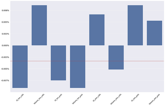

Image by Author

Conclusion

I hope you enjoyed this article! This API can be extremely valuable if utilized correctly. I encourage the reader to try this out with other stocks and/or explore other metrics that could help isolate unusual options activity. Also, consider your risks when trading options; they can be much more volatile than stocks alone, so I suggest educating yourself as much as possible and trading in a simulated environment as you decide which strategy works best for you.

Disclaimer

Trading options involves significant risk and is not suitable for all investors. Options trading can result in substantial financial losses, and past performance is not necessarily indicative of future results. Before engaging in options trading, it’s essential to understand the risks involved and carefully consider your investment objectives, level of experience, and risk tolerance.

The information provided in this article is for educational purposes only and should not be construed as investment advice or a recommendation to buy or sell any financial instrument. The analysis of unusual options data and its potential impact on next day returns is based on historical data and hypothetical scenarios. Actual results may vary, and there is no guarantee of success in trading options or any financial market.

I am not a professional financial advisor or licensed broker, and I do not provide personalized investment advice. Any decisions you make based on the information presented in this article are solely your responsibility. It’s strongly recommended to consult with a qualified financial advisor or professional before making any investment decisions.

Visit us at DataDrivenInvestor.com

Subscribe to DDIntel here.

Featured Article:

Singapore: Unveiling a Tapestry of Possibilities and Global Connections | DataDrivenInvestor

Introducing Singapore's Fund Platform | DataDrivenInvestor

Join our creator ecosystem here.

DDI Official Telegram Channel: https://t.me/+tafUp6ecEys4YjQ1

Follow us on LinkedIn, Twitter, YouTube, and Facebook.